13.8 Multicollinearity | Econometrics I

13.8.1 The problem

Collinearity: High correlation exists among two or more independent variables.
This means the correlated variables contribute redundant information to the multiple regression model.
Including two highly correlated explanatory variables can adversely affect the regression results:
1. No new information provided
2. Can lead to unstable coefficients (large standard error and low t-values)
3. Coefficient signs may not match prior expectations

Multiple linear regression assumes that there is no multicollinearity in the data.

Multicollinearity occurs when the independent variables are too highly correlated with each other.

After reading this Section you will be able to:

Identify collinearity in multiple linear regression.
Understand the effect of collinearity on regression models.

13.8.2 Exact collinearity

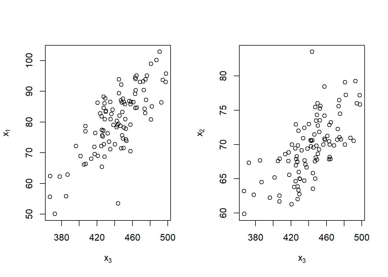
Let’s create a dataset where one of the predictors, \(x_3\), is a linear combination of the other predictors, \(x_1\) and \(x_2\):

\[x_3 = 2 \times x_1 + 4 \times x_2 + 3\]

Dataset
\(y\)	\(x_1\)	\(x_2\)	\(x_3\)
170.7135	93.70958	76.00483	494.4385
152.9106	74.35302	75.22376	452.6011
152.7866	83.63128	64.98396	430.1984
170.6306	86.32863	79.24241	492.6269
152.3320	84.04268	66.66613	437.7499
151.3155	78.93875	70.52757	442.9878

What happens when we attempt to fit a regression model using all of the predictors?

\[y_i = \beta_0 +\beta_1x_{1i}+\beta_2x_{2i}+\beta_3x_{3i}+\epsilon_i\]

. 
. Call:
. lm(formula = y ~ x1 + x2 + x3, data = exact_collin_data)
. 
. Residuals:
.      Min       1Q   Median       3Q      Max 
. -2.57662 -0.66188 -0.08253  0.63706  2.52057 
. 
. Coefficients: (1 not defined because of singularities)
.             Estimate Std. Error t value Pr(>|t|)    
. (Intercept) 2.957336   1.735165   1.704   0.0915 .  
. x1          0.985629   0.009788 100.702   <2e-16 ***
. x2          1.017059   0.022545  45.112   <2e-16 ***
. x3                NA         NA      NA       NA    
. ---
. Signif. codes:  0 '***' 0.001 '**' 0.01 '*' 0.05 '.' 0.1 ' ' 1
. 
. Residual standard error: 1.014 on 97 degrees of freedom
. Multiple R-squared:  0.9923,  Adjusted R-squared:  0.9921 
. F-statistic:  6236 on 2 and 97 DF,  p-value: < 2.2e-16

When this happens, we say there is exact collinearity in the dataset.

As a result of this issue, the software used here \(R\) essentially chose to fit the model without \(x_3\).

. Warning: Model matrix is rank deficient. Parameters x3 were not estimable.

	y
Regressor	\(\hat \beta\)	std. Error	\(t_{stat}\)	\(p\)-value
(Intercept)	2.96	1.74	1.70	0.0915
x1	0.99	0.01	100.70	<0.001
x2	1.02	0.02	45.11	<0.001
Observations	100
R² / R² adjusted	0.992 / 0.992

However notice what two other models would accomplish exactly the same fit:

Model 1: \(y_i = \beta_0 +\beta_1x_{1i}+\beta_2x_{2i}+\epsilon_{i1}\)
Model 2: \(y_i = \beta_0 +\beta_1x_{1i}+\beta_3x_{3i}+\epsilon_{i2}\)
Model 3: \(y_i = \beta_0 +\beta_2x_{2i}+\beta_3x_{3i}+\epsilon_{i3}\)

	y			y			y
Variable	Estimates	std. Error	p-value	Estimates	std. Error	p-value	Estimates	std. Error	p-value
(Intercept)	2.96	1.74	0.092	2.19	1.75	0.213	1.48	1.74	0.398
x1	0.99	0.01	<0.001	0.48	0.02	<0.001
x2	1.02	0.02	<0.001				-0.95	0.03	<0.001
x3				0.25	0.01	<0.001	0.49	0.00	<0.001
Observations	100			100			100
R² / R² adjusted	0.992 / 0.992			0.992 / 0.992			0.992 / 0.992

We can observe that the fitted values for each of the three models are exactly the same. This is a result of \(x_3\) containing all of the information from \(x_1\) and \(x_2\). As long as one of \(x_1\) or \(x_2\) are included in the model, \(x_3\) can be used to recover the information from the variable not included.

Fitted Values (Top 6)
Model 1	Model 2	Model 3
172.6216	172.6216	172.6216
152.7488	152.7488	152.7488
151.4793	151.4793	151.4793
168.6395	168.6395	168.6395
153.5956	153.5956	153.5956
152.4923	152.4923	152.4923

While their fitted values are all the same, their estimated coefficients are wildly different. The sign of \(x_2\) is switched in two of the models! So only Model 1 properly explains the relationship between the variables, Model 2 and Model 3 still predict as well as Model 1 despite the coefficients having little to no meaning¹⁰, since the real model used to generate the dataset is:

\[ y_i = 3 + x_{1i}+ x_{2i}+ \epsilon_i, \epsilon_i \sim N(0,1)\]

Exact collinearity is an extreme example of collinearity, which occurs in multiple regression when predictor variables are highly correlated. Collinearity is often called multicollinearity, since it is a phenomenon that really only occurs during multiple regression.

13.8.3 Indicators of Multicollinearity

Coefficients differ from the values expected by theory or experience, or have incorrect signs.
Coefficients of variables believed to be a strong influence have small \(t\) statistics indicating that their values do not differ from 0.
All the coefficient student \(t\) statistics are small, indicating no individual effect, but the overall \(F\) statistic indicates a strong effect for the total regression model.
High correlations exist between individual independent variables or one or more of the independent variables have a strong linear regression relationship to the other independent variables or a combination of both.

13.8.4 Detecting Multicollinearity

Examine the simple correlation matrix to determine if strong correlation exists between any of the model independent variables.
Look for a large change in the value of a previous coefficient when a new variable is added to the model.
Does a previously significant variable become insignificant when a new independent variable is added?
Does the estimate of the standard deviation of the model increase when a variable is added to the model?

13.8.5 Corrections for Multicollinearity

Remove one or more of the highly correlated independent variables.
Change the model specification, including possibly a new independent variable that is a function of several correlated independent variables.
Obtain additional data that do not have the same strong correlations between the independent variables.

13.8.6 Our Monet Case

Using the Case described in @ref{monet}, we use Multiple Linear Regression to model the relationship between PRICE and the rest of variables in the dataset.

Data on Sales of Monet Paintings
PRICE	HEIGHT	WIDTH	SIGNED	PICTURE	HOUSE
3.993780	21.3	25.6	1	1	1
8.800000	31.9	25.6	1	2	2
0.131694	6.9	15.9	0	3	3
2.037500	25.7	32.0	1	4	2
5.282500	25.5	35.6	1	5	1
2.530000	25.6	36.4	1	6	2
0.364343	25.6	36.2	1	7	2
2.723870	31.9	39.4	1	8	2
3.520000	23.6	31.9	1	9	1
0.497500	19.5	25.0	1	10	2
Note: One price per painting. Only first 10 observations.

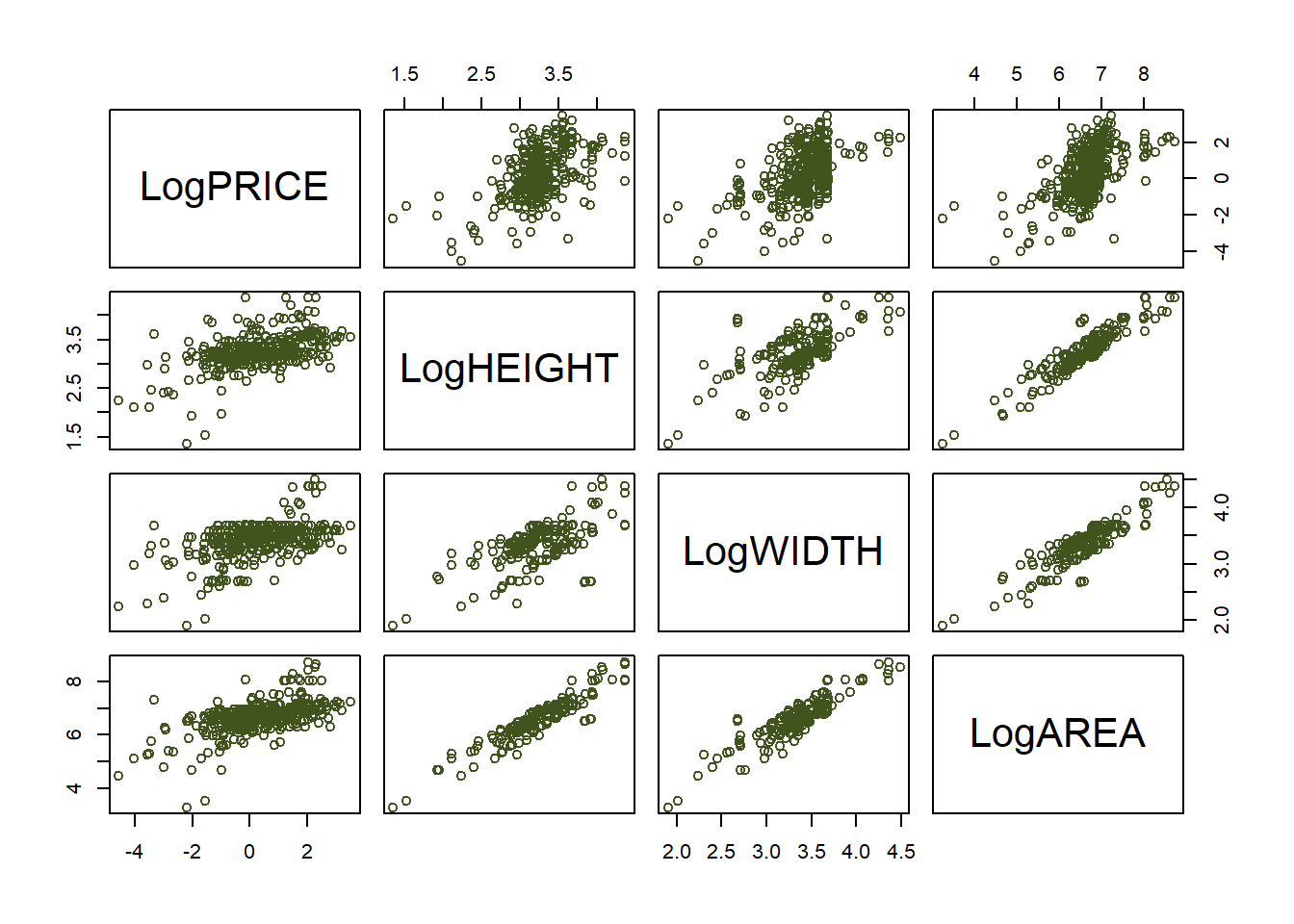
Figure 13.1: Graphical visualization of the correlation matrix

Pairwise Correlations
	LogPRICE	LogHEIGHT	LogWIDTH	LogAREA
LogPRICE	1.000	0.528	0.504	0.578
LogHEIGHT	0.528	1.000	0.599	0.907
LogWIDTH	0.504	0.599	1.000	0.880
LogAREA	0.578	0.907	0.880	1.000

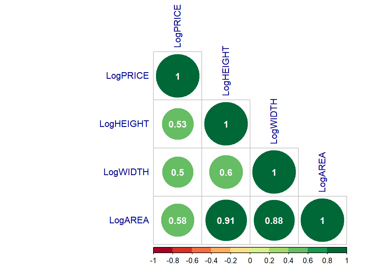
Figure 13.2: Graphical visualization of the correlation matrix

The matrix above returns all pairwise correlations. Notice this is a symmetric matrix. Recall that correlation measures strength and direction of the linear relationship between to variables. The correlation between LogHEIGHT and LogAREA is extremely high, as well as the correlation between LogWIDTH and LogAREA.

Unlike exact collinearity, here we can still fit a model with all of the predictors, but what effect does this have?

Model 0: \(\text{LogPRICE}_i = \beta_0 + \beta_1\text{LogHEIGHT}_i + \beta_2\text{LogWIDTH}_i+ \beta_3\text{LogAREA}_i+\epsilon_{i0}\)

. 
. Call:
. lm(formula = LogPRICE ~ ., data = dataset)
. 
. Residuals:
.     Min      1Q  Median      3Q     Max 
. -4.4778 -0.7111 -0.0832  0.7627  2.9904 
. 
. Coefficients: (1 not defined because of singularities)
.             Estimate Std. Error t value Pr(>|t|)    
. (Intercept)  -8.4336     0.6569 -12.839  < 2e-16 ***
. LogHEIGHT     1.3545     0.2028   6.678 8.79e-11 ***
. LogWIDTH      1.2709     0.2284   5.565 5.01e-08 ***
. LogAREA           NA         NA      NA       NA    
. ---
. Signif. codes:  0 '***' 0.001 '**' 0.01 '*' 0.05 '.' 0.1 ' ' 1
. 
. Residual standard error: 1.11 on 373 degrees of freedom
. Multiple R-squared:  0.334,   Adjusted R-squared:  0.3305 
. F-statistic: 93.54 on 2 and 373 DF,  p-value: < 2.2e-16

Although the \(F-\)test for the regression tells us that the regression is significant, the parameter of LogAREA can not be defined because of singularities. Therefore, we fit alternative models:

Model 1: \(\text{LogPRICE}_i = \beta_0 + \beta_1\text{LogHEIGHT}_i+ \beta_2\text{LogWIDTH}_i+\epsilon_{i1}\)
Model 2: \(\text{LogPRICE}_i = \beta_0 + \beta_1\text{LogHEIGHT}_i+ \beta_3\text{LogAREA}_i+\epsilon_{i2}\)
Model 3: \(\text{LogPRICE}_i = \beta_0 + \beta_2\text{LogWIDTH}_i+ \beta_3\text{LogAREA}_i+\epsilon_{i3}\)

	Log PRICE			Log PRICE			Log PRICE
Variable	Estimates	std. Error	p-value	Estimates	std. Error	p-value	Estimates	std. Error	p-value
(Intercept)	-8.43	0.66	<0.001	-8.43	0.66	<0.001	-8.43	0.66	<0.001
LogHEIGHT	1.35	0.20	<0.001	0.08	0.39	0.829
LogWIDTH	1.27	0.23	<0.001				-0.08	0.39	0.829
LogAREA				1.27	0.23	<0.001	1.35	0.20	<0.001
Observations	376			376			376
R² / R² adjusted	0.334 / 0.330			0.334 / 0.330			0.334 / 0.330

One of the first things we should notice is that parameters of LogHEIGHT and LogWIDTH have a large change in the value and they are not significant when LogAREA is included as regressor in the same model (Model 2 and Model 3).

Another interesting result is the opposite signs of the coefficient for LogWIDTH in Model 1 and Model 2. This should seem rather counter-intuitive. Increasing WIDTH increases or decreases PRICE?

Moreover, the value of the parameter of LogAREA in Model 2 is similar to the value of the parameter of LogWIDTH in Model 1. The value of the parameter of LogAREA in Model 2 is similar to the value of the parameter of LogHEIGHT in Model 1.

This happens as a result of the predictors being highly correlated.

When LogAREA and LogHEIGHT are both in the model, their effects on the response are lessened individually, but together they still explain a large portion of the variation of LogPRICE .

Another way to inspect for Multicollineary is using regressions between regressors, like:

Model A1: \(\text{LogAREA}_i = \alpha_0 + \alpha_1 \text{LogHEIGHT}_i + e_{i1}\)
Model A2: \(\text{LogAREA}_i = \alpha_0 + \alpha_2 \text{LogWIDTH}_i + e_{i2}\)

	Log AREA			Log AREA
Variable	Estimates	std. Error	p-value	Estimates	std. Error	p-value
(Intercept)	1.69	0.12	<0.001	0.95	0.16	<0.001
LogHEIGHT	1.53	0.04	<0.001
LogWIDTH				1.67	0.05	<0.001
Observations	376			376
R² / R² adjusted	0.823 / 0.822			0.775 / 0.774

13.8.7 Revisiting Monet Case

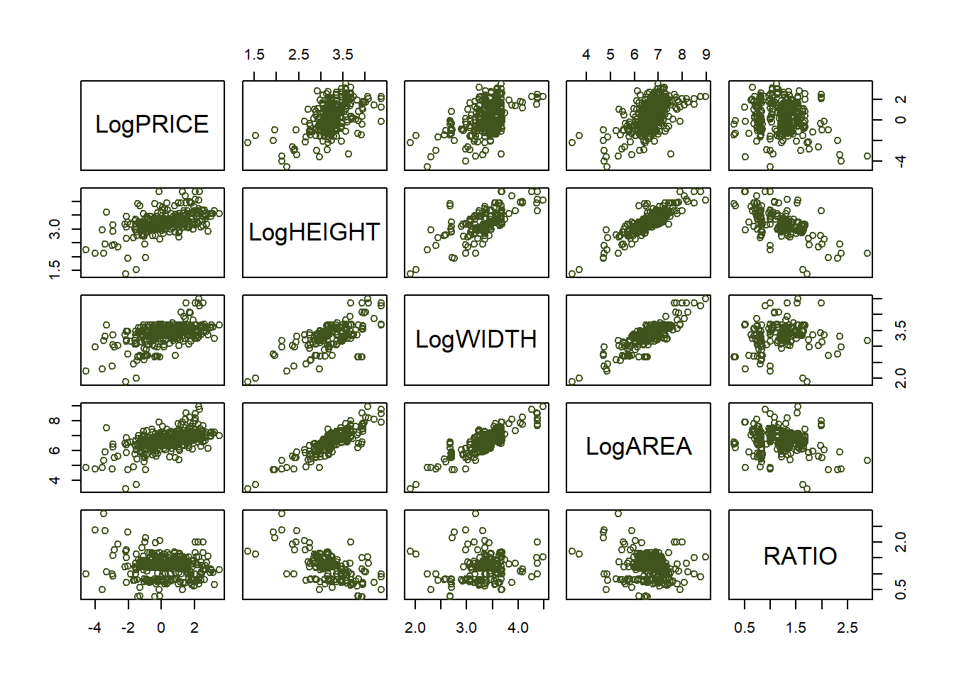
For illustrative purposes, we add a small random noise to the variable AREA - that is, AREA is not an exact combination of HEIGHT and WIDTH - and we create a new variable: RATIO.

\[\begin{align} \text{LogAREA}=\log ( WIDTH \times HEIGHT) + \varepsilon; \,\,\, \varepsilon \sim N(0,0.2) \end{align}\]

\[\begin{align} \text{RATIO}= \dfrac{WIDTH}{HEIGHT} \end{align}\]

Pairwise Correlations
	LogPRICE	LogHEIGHT	LogWIDTH	LogAREA	RATIO
LogPRICE	1.000	0.528	0.504	0.551	-0.162
LogHEIGHT	0.528	1.000	0.599	0.855	-0.577
LogWIDTH	0.504	0.599	1.000	0.839	0.272
LogAREA	0.551	0.855	0.839	1.000	-0.187
RATIO	-0.162	-0.577	0.272	-0.187	1.000

Model 1: \(\text{LogPRICE}_i = \beta_0 + \beta_1\text{LogHEIGHT}_i \epsilon_{i1}\)
Model 2: \(\text{LogPRICE}_i = \beta_0 + \beta_2\text{LogWIDTH}_i + \epsilon_{i2}\)
Model 3: \(\text{LogPRICE}_i = \beta_0 + \beta_3\text{LogAREA}_i + \epsilon_{i3}\)
Model 4: \(\text{LogPRICE}_i = \beta_0 + \beta_1\text{LogHEIGHT}_i + \beta_2\text{LogWIDTH}_i+ \beta_3\text{LogAREA}_i + \epsilon_{i4}\)
Model 5: \(\text{LogPRICE}_i = \beta_0 + \beta_1\text{LogHEIGHT}_i + \beta_3\text{LogAREA}_i + \epsilon_{i5}\)
Model 6: \(\text{LogPRICE}_i = \beta_0 + \beta_2\text{LogWIDTH}_i+ \beta_3\text{LogAREA}_i + \epsilon_{i6}\)

	Log PRICE			Log PRICE			Log PRICE
Variable	Estimates	std. Error	p-value	Estimates	std. Error	p-value	Estimates	std. Error	p-value
(Intercept)	-6.29	0.55	<0.001	-7.15	0.66	<0.001	-7.72	0.63	<0.001
LogHEIGHT	2.03	0.17	<0.001
LogWIDTH				2.18	0.19	<0.001
LogAREA							1.21	0.09	<0.001
Observations	376			376			376
R² / R² adjusted	0.279 / 0.277			0.254 / 0.252			0.304 / 0.302

	Log PRICE			Log PRICE			Log PRICE
Variable	Estimates	std. Error	p-value	Estimates	std. Error	p-value	Estimates	std. Error	p-value
(Intercept)	-8.44	0.66	<0.001	-7.73	0.63	<0.001	-8.09	0.66	<0.001
LogHEIGHT	1.28	0.35	<0.001	0.81	0.32	0.011
LogWIDTH	1.20	0.37	0.001				0.62	0.34	0.073
LogAREA	0.07	0.29	0.804	0.81	0.18	<0.001	0.94	0.17	<0.001
Observations	376			376			376
R² / R² adjusted	0.334 / 0.329			0.316 / 0.312			0.310 / 0.306

Including RATIO:

Model 7: \(\text{LogPRICE}_i = \beta_0 + \beta_4\text{RATIO}_i \epsilon_{i7}\)
Model 8: \(\text{LogPRICE}_i = \beta_0 + \beta_3\text{LogAREA}_i + \beta_4\text{RATIO}_i + \epsilon_{i8}\)
Model 9: \(\text{LogPRICE}_i = \beta_0 + \beta_1\text{LogHEIGHT}_i + \beta_4\text{RATIO}_i + \epsilon_{i9}\)

	Log PRICE			Log PRICE			Log PRICE
Variable	Estimates	std. Error	p-value	Estimates	std. Error	p-value	Estimates	std. Error	p-value
(Intercept)	1.14	0.27	<0.001	-7.24	0.72	<0.001	-8.92	0.85	<0.001
RATIO	-0.67	0.21	0.002	-0.25	0.18	0.165	0.89	0.22	<0.001
LogAREA				1.18	0.10	<0.001
LogHEIGHT							2.51	0.20	<0.001
Observations	376			376			376
R² / R² adjusted	0.026 / 0.024			0.307 / 0.303			0.309 / 0.306

References:

Adapted from Statistics for Business and Economics Chapter 13. Additional Topics in Regression Analysis. Copyright (c) 2013 Pearson Education.
Examples taken from Applied Statistics with R