6.6 Comparing Group Means
Let’s examine the difference between the mean price of the signed and non-signed paintings.
Is the difference in mean price statistically significant?
The field of statistical inference consists of those methods used to make decision or to draw conclusions about a population.
Statistical inference may be divided into two major areas: parameter estimation and hypothesis testing.
One of the most common tests in statistics, the t-test, is used to determine whether the means of two groups are equal to each other.
- The assumption for the test is that both groups are sampled from normal distributions with equal variances.
- The null hypothesis is that the two means are equal, and the alternative is that they are not.
- It is known that under the null hypothesis, we can calculate a t-statistic that will follow a t-distribution with \(n_1+n_2-2\) degrees of freedom.
Preliminary test to check t-test assumptions:
- Is this a large sample? ¿\(n < 30\)?
- If the sample size is not large enough (less than 30, central limit theorem), we need to check whether the data follow a normal distribution.
How to check the normality?
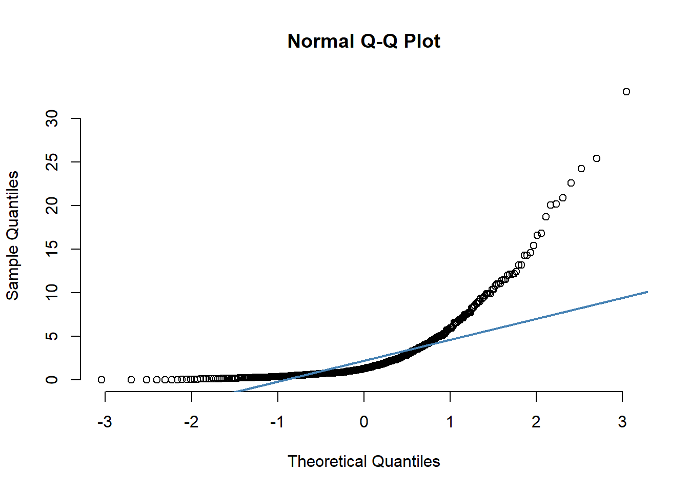
We can perform visual inspection of the data normality using Q-Q plots (quantile-quantile plots). Q-Q plot draws the correlation between a given sample and the normal distribution.
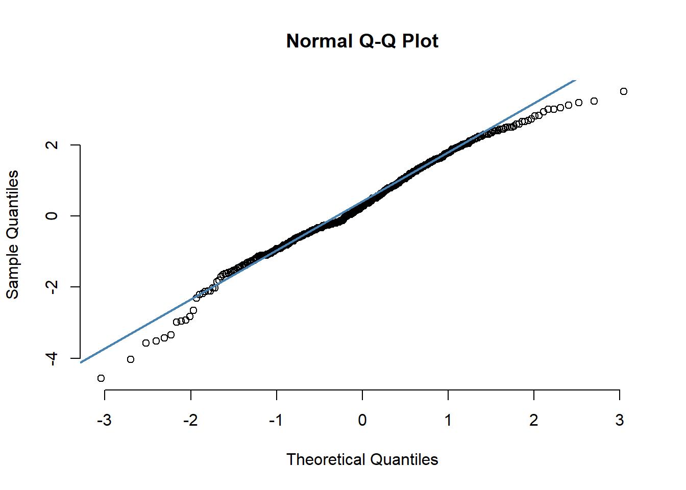
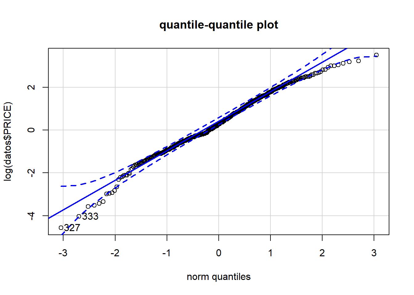
. [1] 327 333As all the points fall approximately along this reference line, we can assume normality.
The normality condition is important for various statistical procedures. And so, it is very important to check if the normality condition is satisfied by the data points, especially in residual analysis. One of the methods to do this is by plotting the Quantile-Quantile Plot.
A quantile is where a sample is divided into equal-sized, adjacent, subgroups. So, if we have a 0.3 quantile, then 30% of the data points lie below the 0.3 quantile and the rest 70% will lie above it. The median is the 0.5 quantile in a dataset.
In the X-axis of the Q-Q plot, we have the theoretical quantiles of a proper normally distributed population and on the Y-axis, the ordered quantiles of our sample data are listed. If both the values of theoretical and sample quantiles are almost equal, then they will lie along a 45° intended line, and we can confirm that the data comes from a normally distributed population. If they do not come from a similar population, their quantiles will also be different from each other.
Adapted from here
6.6.1 Decision Making for Single Sample
The mean price differs from … ?
\[H_0: \mu = 3.30 \] \[H_1: \mu \not= 3.30 \]
.
.   One Sample t-test
.
. data:  log(datos$PRICE)
. t = -45.57, df = 429, p-value < 2.2e-16
. alternative hypothesis: true mean is not equal to 3.3
. 95 percent confidence interval:
.  0.2047561 0.4607211
. sample estimates:
. mean of x
. 0.3327386
.
. One Sample t-test
.
. data: log(datos$PRICE)
. t = 0.042058, df = 429, p-value = 0.9665
. alternative hypothesis: true mean is not equal to 0.33
. 95 percent confidence interval:
. 0.2047561 0.4607211
. sample estimates:
. mean of x
. 0.3327386Let \(X_1,X_2,\ldots,X_n\) be a random sample for a normal distribution with unknown mean \(\mu\) and unknown variance \(\sigma^2\). The quantity
\[T=\dfrac{\bar{X}-\mu}{S/\sqrt{n}}\]
has a \(t\) distribution \(n-1\) degrees of freedom.
6.6.2 Decision Making for Two Samples
\[H_0: \mu_1 - \mu_2 = 0 \] \[H_1: \mu_1 - \mu_2 \not= 0 \]
| count | mean | sd |
|---|---|---|
| 430 | 3.089996 | 4.31126 |
| count | mean | sd |
|---|---|---|
| 430 | 0.3327386 | 1.350237 |
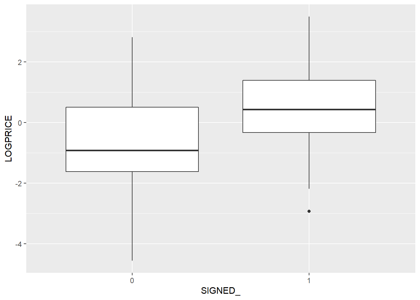
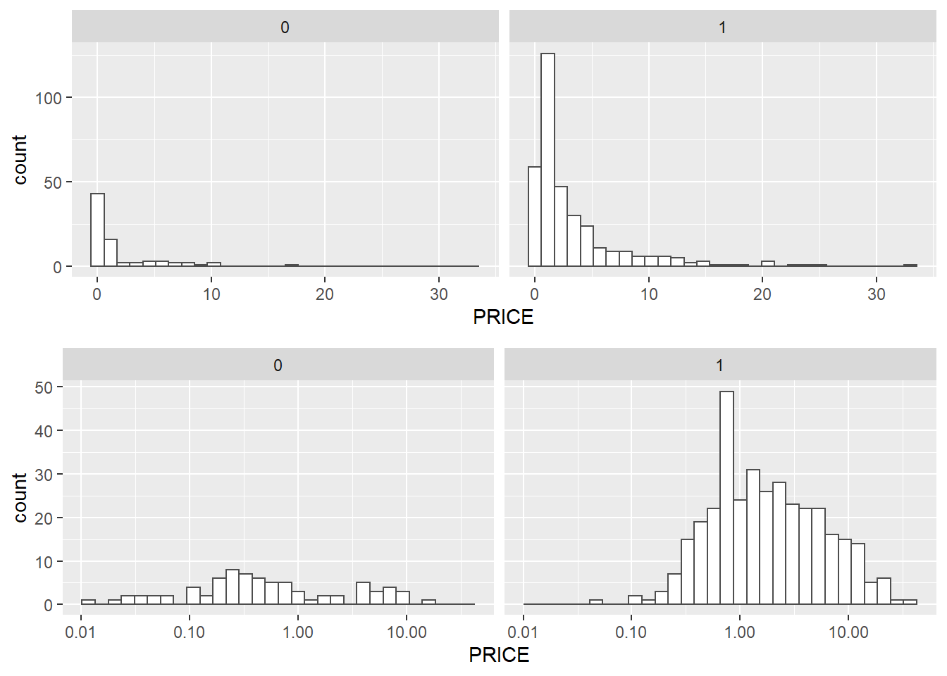
Do we see similar skewness within the sample distributions?
.
.   Welch Two Sample t-test
.
. data:  LOGPRICE by SIGNED
. t = -5.9926, df = 92.131, p-value = 3.967e-08
. alternative hypothesis: true difference in means is not equal to 0
. 95 percent confidence interval:
.  -1.6142628 -0.8106198
. sample estimates:
. mean in group 0 mean in group 1
. -0.6625911 0.5498502- \(X_{11},X_{12},\ldots,X_{1n_1}\) is a random sample of size \(n_1\) from population \(1\)
- \(X_{21},X_{22},\ldots,X_{2n_2}\) is a random sample of size \(n_2\) from population \(2\)
- The two populations represented by \(X_1\) and \(X_2\) are independent.
- Both population are normal.
The quantity
\[T=\dfrac{\bar{X}_1 - \bar{X}_2 - (\mu_1 - \mu_2)}{S_p \sqrt{\frac{1}{n_1}+\frac{1}{n_2}}}\]
has a \(t\) distribution \(n_1 + n_2 - 2\) degrees of freedom.