12.7 Coefficient of Determination
How much does the relationship between advertising and sales help us understand and predict sales? We’d like to be able to quantify the predictive power of the relationship in determining sales levels. How much more do we know about sales thanks to the advertising data?
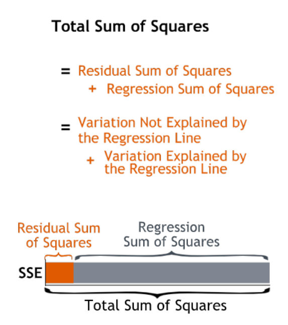
The difference between the Total Sum of Squares and the Residual Sum of Squares, 6.88 trillion in this case, is called the Regression Sum of Squares. The Regression Sum of Squares measures the variation in sales explained by the regression line.
A standardized measure of the regression line’s explanatory power is called R-squared. R-squared is the fraction of the total variation in the dependent variable that is explained by the regression line.
R-squared will always be between 0 and 1 — at worst, the regression line explains none of the variation in sales; at best it explains all of it.
We find R-squared by dividing the variation explained by the regression line — the Regression Sum of Squares — by the total variation in the dependent variable — the Total Sum of Squares.
\[\begin{equation} R^2 = \dfrac{\text{Variation explained by Regression}}{\text{Total Variation}}=\dfrac{\text{Regression Sum of Squares}}{\text{Total Sum of Squares}} \end{equation}\]
12.7.1 Technical notes
The coefficient of determination is a measure of the amount of variability in the data accounted for by the regression model. The total variability of the data is measured by the total sum of squares, \(SS_T\). The amount of this variability explained by the regression model is the regression sum of squares, \(SS_R\). The coefficient of determination is the ratio of the regression sum of squares to the total sum of squares.
\[R^2 = \dfrac{SS_R}{SS_T}\,\]
\(R^2\) can take on values between 0 and 1.
The denominator is the total sum of squares (abbreviated \(SS_T\)). It is the sum of the square of deviations of all the observations, \(y_i\), from their mean, \(\bar{y}\).
\[S{{S}_{T}}=\underset{i=1}{\overset{n}{\mathop \sum }}\,{{({{y}_{i}}-\bar{y})}^{2}}\,\] This term is the numerator of the total variance (i.e., the variance of all of the observed data) or the variance estimated using the observed data.
When you attempt to fit a regression model to the observations, you are trying to explain some of the variation of the observations using this model. If the regression model is such that the resulting fitted regression line passes through all of the observations, then you would have a “perfect” model. In this case the model would explain all of the variability of the observations. Therefore, the model sum of squares (also referred to as the regression sum of squares and abbreviated \(SS_R\)) equals the total sum of squares; i.e., the model explains all of the observed variance:
\[ SS_R=SS_T \]
For the perfect model, the regression sum of squares, \(SS_R\), equals the total sum of squares, \(SS_T\), because all estimated values, \(\hat{y}_i\), will equal the corresponding observations, \(y_i\). \(SS_R\) can be calculated using a relationship similar to the one for obtaining \(SS_T\) by replacing \(y_i\) by \(\hat{y}_i\) in the relationship of \(SS_T\). Therefore:
\[S{{S}_{R}}=\underset{i=1}{\overset{n}{\mathop \sum }}\,{{({{\hat{y}}_{i}}-\bar{y})}^{2}}\,\]
- Since \(R^2\) is a proportion, it is always a number between 0 and 1.
- If \(R^2=1\), all of the data points fall perfectly on the regression line. The predictor \(x\) accounts for all of the variation in \(y\).
- If \(R^2=0\), the estimated regression line is perfectly horizontal. The predictor \(x\) accounts for none of the variation in \(y\).