12.4 Calculating the Regression Line
To quantify how accurately a line fits a data set, we measure the vertical distance between each data point and the line.
We measure vertical distance because we are interested in how well the line predicts the value of the dependent variable. The dependent variable — in our case, sales — is measured on the vertical axis. For each data point, we want to know how close the value of sales predicted by the line is to the historically observed value of sales.
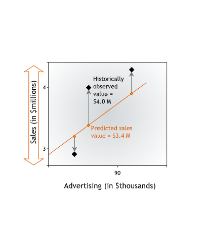
From now on we will refer to this vertical distance between a data point and the line as the error in prediction or the residual error, or simply the error. The error is the difference between the observed value and the line’s prediction for our dependent variable. This difference may be due to the influence of other variables or to plain chance.
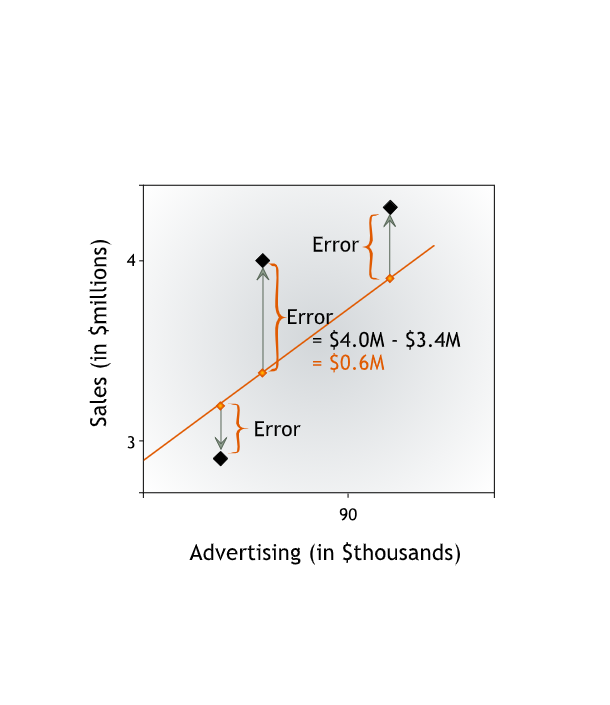
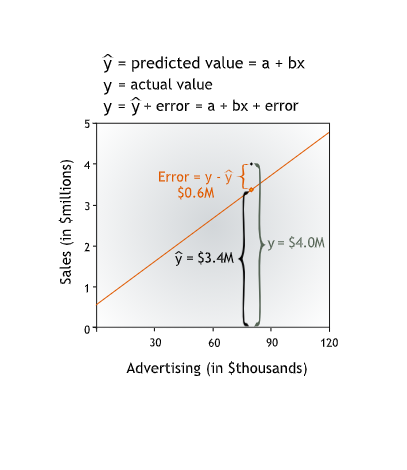
Going forward, we will refer to the value of the dependent variable predicted by the line as y-hat and to the actual value of the dependent variable as y. Then the error is y - (y-hat), the difference between the actual and predicted values of the dependent variable.
For each line, we can calculate the Sum of Squared Errors to determine its accuracy.
The lower the Sum of Squared Errors, the more precisely the line fits the data, and the higher the line’s accuracy.
The line that most accurately describes the relationship between advertising and sales — the regression line — is the line that minimizes the sum of squares. The line that most accurately fits the data — the regression line — is the line for which the Sum of Squared Errors is minimized.
12.4.1 Technical Note: the “Best Fitting Line”
In light of the least squares criterion, which line do you now think is the best fitting line?
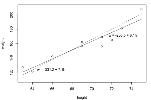
The following two side-by-side tables illustrate the implementation of the least squares criterion for the two lines up for consideration — the dashed line and the solid line.
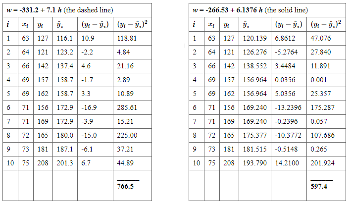
Based on the least squares criterion, which equation best summarizes the data? The sum of the squared prediction errors is 766.5 for the dashed line, while it is only 597.4 for the solid line. Therefore, of the two lines, the solid line, \(w = -266.53 + 6.1376h\), best summarizes the data. But, is this equation guaranteed to be the best fitting line of all of the possible lines we didn’t even consider?
In order to answer thw question we should find the same result for an infinite number of possible lines — clearly, an impossible task! Fortunately, somebody has done some dirty work for us by figuring out formulas for the intercept \(\beta_0\) and the slope \(\beta_1\) for the equation of the line that minimizes the sum of the squared prediction errors.
The formulas are determined using methods of calculus. We minimize the equation for the sum of the squared prediction errors:
\[Q=\sum_{i=1}^{n}(y_i-(\beta_0+\beta_1x_i))^2\] (that is, take the derivative with respect to \(\beta_0\) and \(\beta_1\), set to \(0\), and solve for b0 and b1) and get the “least squares estimates” for \(\beta_0\) and \(\beta_1\):
\[\hat{\beta}_1 = \dfrac{ \sum^n_{i = 1} x_i y_i - n \bar{x} \bar{y}}{\sum^n_{i = 1} (x_i - \bar{x})^2}\]
\[\hat{\beta}_0 = \bar{y} - \hat{\beta}_1 \bar{x}\] Because the formulas for \(\beta_0\) and \(\beta_1\) are derived using the least squares criterion, the resulting equation — \(\hat{y}_i=\beta_0+\beta_1x_i\) — is often referred to as the “least squares regression line,” or simply the “least squares line.” It is also sometimes called the “estimated regression equation.”
Source: here